This lab has four parts: Parts A to D. The four parts together form a sequence of tasks. These parts are not independent and should be done one after another.
You need to show your tutors all the four parts. Remember you must be ready for some assessment half an hour before the end of the class. These three exercises are worth 2 marks.
For all the programs, we expect that you choose informative variable names and document your program. There is also an online assessment question which is worth 1 mark. We suggest that you attempt this question after completing all the parts.You should make a directory called lab09 to store your files for this lab.
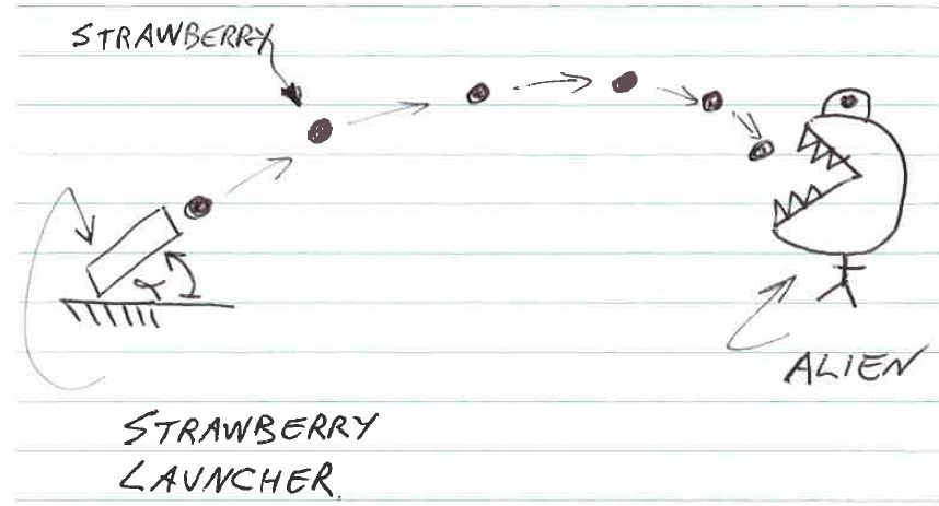
Remark: The real-life application of this problem is missiles. For this lab, let us be innocent and consider strawberries and aliens instead.
The starting point of simulation is mathematical modelling. In ENGG1811, we will always give you the mathematical models. After you have learned enough knowledge in your own discipline, you will be able to come out with your own mathematical model for the work that you do.
The motion of the strawberries in the air is affected by two factors: gravitational pull and air resistance. A common model for air resistance is that the resistive force is proportional to total speed of the object. We assume the launcher, strawberries and alien live in a two-dimension space. The horizontal direction is the x-direction and the vertical direction is the y-direction. The position of the strawberry is therefore defined by its x- and y-coordinates. We use px(t) and py(t) to denote the x- and y-coordinates of the strawberry at time t. In addition, we use vx(t) and vy(t) to denote the velocity of the strawberry in x- and y-directions. The motion of the strawberry obeys the following set of ordinary differential equations:

where m and c are, respectively, the mass and drag coefficient; and g is the acceleration due to gravity. Since the strawberry has an x- and a y-component in velocity, its total speed is given by the square root of (vx(t)2 + vy(t)2). If you are interested, Equations (3) and (4) are derived from Newton's Second Law. Equation (3) says that the strawberry experiences resistance as it moves in the air in the x-direction. Equation (4) says that the strawberry experiences both gravitational pull and air resistance when it moves in the y-direction.
Given Equations (1)-(4), you can use Euler's forward rule to derive how to calculate the position and velocity at time t + Δ from that at time t. We have derived the equations for you, as follows:

def
sim_projectile(time_array,m,c,v0,theta0d):
return position_x,
position_y
where time_array is a 1-D numpy array containing time instances, m is mass, c is drag coefficient, v0 is initial launch speed, theta0d is launch angle in degrees. This function returns two outputs, which are the x- and y-coordinates at the corresponding time instances specified by the numpy array time_array.
The function is missing two lines of code (within the for-loop located near the end of the function), which are the two Python statements for updating position_y and velocity_y. You are asked to fill in these two statements at the places indicated. You may wish to read the function to see what it does. In particular, note that v0 is the initial total speed, which means the initial speed in the x- and y-directions, are, respectively v0*math.cos(math.radians(theta0d)) and v0*math.sin(math.radians(theta0d)).
After you have completed this, you can test the function by using the Python script test_sim_projectile.py. Take a look at what the script does. It defines the problem and simulation parameters, as follows:
The simulation in Part A allows you to determine the trajectory of the strawberry launched at a given speed and angle. Let us now assume that the alien is located at a height (y-coordinate) of +10, and the alien's can only swallow the strawberries when they are falling down. The trajectory plot in Part A shows that, with a launch angle of 35 degrees, a rough estimate of the landing position of the strawberries will be at the coordinates (96,10). This position is obtained from using visual inspection from the graph. Your task for this Part is to use Python to automatically determine the landing position (assuming a landing height of 10) as well as the time to reach the landing position, from the trajectories computed in Part A.We will define the exact meaning of landing using an example in a moment.
We will give you some idea how you can use Python to find the landing time and position. The trajectory has 101 numbers so it may be hard to work with. So we will use a small example to illustrate the method. This is a typical problem solving technique. If you can solve the problem for a small example, then you can transfer the solution to a larger instance of the problem. Let us assume that you have three arrays px, py and tv, which have analogous meaning to position_x, position_y and time_array that we have used above. We made up some values for the elements of these three arrays:
tv = np.array([ 0.6, 0.7, 1.5, 1.6, 1.7, 1.8, 1.9])
px = np.array([ 2.4, 2.9, 5.7, 6.6, 7.5, 8.4, 9.3])
py = np.array([ 9.7, 10.1, 10.5, 10.2, 10.1, 9.9, 9.8])
Note that this example contains the main feature of the problem with the positions in the y-direction dropping from a value above 10 to a value below 10. It means that at some point in time, the strawberry has a height of exactly 10. Instead of determining the exact time of crossing, we use an approximation here. First, we consider only the time instances in the array tv. Second, we say that landing occurs at time t if the vertical position of the strawberry at time t is closest to the level of 10, but is still at or above the level of 10. For this example, landing occurs at time instance 1.7 because the strawberry is just above the level 10, at a height of 10.1 to be specific. At the next time instance, at time 1.8, the strawberry is below the level of 10, at 9.9 to be specific. This is not exact, but if the time increment is small, the error will not be big. (This is also on the condition that the alien opens its mouth wide!) We say that the landing distance (which measures position in the x-direction) is 7.5 and the landing time is 1.7.
We suggest that you work with this example first to find out what Python statements you need to determine the landing distance and landing time from tv, px and py. Once you get this going, you can test whether it works for the time_array, position_x and position_y. If you want some more hint, you can click here.
You can use any method to solve this problem as long as it can be automated. Having done some programming, you may think that you need some loops and if statements to solve this problem. Yes, you can do that, but I want to say that this problem has some special features and you can solve this problem using the Python numpy functions numpy.where() and numpy.max(). We discussed these two functions in Week 6's lecture on numpy, see the sample code in numpy_max.py and numpy_where.py which are filed under code_prelim_6A in Week 6's lecture. You can also find examples of using these two functions in the sample code numpy_max_final.py and numpy_logic_final.py which are filed under code_final_6A in Week 6's lecture.
You should try to do this Part using a script, because you will need to write a function to do these steps in Part C. You can keep the script to show your tutor.
Once you have got Part B working, you should write a function to determine the landing distance and landing time (these are the outputs) from the 1-d arrays time_array, position_x and position_y and a scalar landing_level (these are the inputs). Note that landing_level is 10 but we should try to make the function general so that it can work with any landing level.
The first and last line of your function should look like:
def find_landing_pos_time(time_array,position_x,position_y,landing_level):
return landing_position, landing_time
You can insert your code in the file sim_projectile.py.
The outline for the function can be seen in the
sim_projectile.py file under your sim_projectile function. Un-comment this
section and then write your code in the space.
You can test your find_landing_position_time function in the console. Try
running
sim.find_landing_pos_time(time_array,position_x,position_y,10)
in the console and look at the output. Compare it to your graph you made
earlier, does the answer seem correct?
First, let us recap what you have achieved by now.
By combining what you have in Parts A and C, you can determine, for a given launch angle, what the landing position and landing time are. What this means is that, you have all the functions that you need to study how the launch angle impacts on landing position and landing time.
In this part, your task is to write a Python script that does the following:
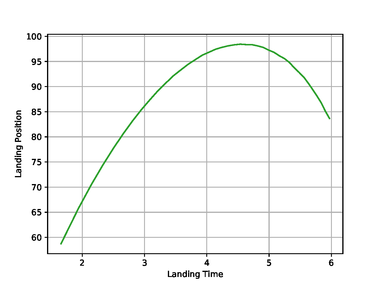
This script does some calculations repeatedly so you need some type of loops (which type?). Once you get your script working, you can plot a graph of landing distance versus landing time. You should get a graph similar to that below.
Let us assume that the alien is at a horizontal distance of 90 from the launcher. You can see from the graph that there are two launch angles that will allow you to feed the alien and one of them will allow you to feed the alien quicker. Your final task is to determine the launch angle to use by using Python statements. You can add these statements to the script and write a Python print statement to display the answer. We do not need a very accurate answer. As long as the launch angle is within 1 degree of the correct value, that is acceptable. You can use any method you like to determine the launch angle. The type of method you used in Part B is also helpful here.
--- Happy feeding! ---
You
should be able to show your tutor the three exercises. You should be
comfortable with using for-loops and
list of lists.
Finally, do not forget to complete your online multiple choice question if you have not done it yet.
If you have completed everything, please do not forget to logout. Simply double click on the "Log Out" icon