- Due date: 5pm, Friday of Week-10 .
- Late Penalty: Late submissions will be penalised at the rate of 10% per day (including weekends). The penalty applies to the maximum available mark. For example, if you submit 2 days late, maximum available marks is 80% of the assignment marks.
- Submissions will not be accepted after 9am Monday of Week-11.
Change Log
- [03:15pm Sunday 01 Aug] To submit this assignment, go to the Assignment 2 page and click the tab named "Make Submission".
- [06:35pm Monday 19 July] The section "Assignment Conditions" added.
Introduction
This assignment is inspired by the Millennium Bridge in London, England. The Millennium Bridge is a suspension bridge for pedestrians only. Many visitors walked across the bridge in the first day of its opening in 2000. However, these visitors were treated to something unusual. They noticed that, when there were many people on the bridge, the bridge started to sway a lot. You can watch the wobbling of the bridge in this YouTube video. Since the bridge did not sway much if there were few people on the bridge, the authority decided to limit the number of people on the bridge. Eventually, the bridge was closed a few days after its opening. The bridge was re-opened after additional dampers have been put on the bridge, see [1] for a report on how the bridge was stabilised.
Engineers and scientists wanted to understand why the Millennium Bridge started to sway when there were many people on the bridge. You probably have learnt about resonance in your Physics class and you are right to guess that the wobbling had something to do with resonance. However, the baffling part is how pedestrians could have caused resonance to occur. One theory, which was published in [2], is that the pedestrians would synchronise their walking with that the bridge's motion and their synchronised movement caused the bridge to sway more. There are also other theories, such as [3], which disputes the theory proposed in [2].
The aim of this assignment is to give you an opportunity to work on a small-scale engineering problem in Python. The engineering system that you will be working on is the Millennium Bridge motion model from [2]. (Note that we are not claiming that [2] is the correct model. We are merely using the model in [2] in a computing exercise.) You will first develop a Python function to simulate the motion of the bridge due to the pedestrians' movement. After that, you will use the simulation program to try out different modifications that can reduce the amount of swaying. On the whole, this assignment relates computer science to two important aspects of engineering, which are simulation and design.
The key objective of this assignment is to for you to learn and use Python and numpy to solve problems. At the same time, we would like to give the problem an engineering context so that you can get some ideas how computing is used in engineering. Note that we used the word inspired earlier because, for this assignment, we took the liberty to simplify the model in [2] and the engineering design problem.
Learning objectives
This assignment is designed to give you practice in- Applying programming to solve a simple engineering simulation and design problem
- Applying a number of numpy features, which include array, slicing, elementwise computation, built-in functions and others
- To organize programs into modules by using functions
- To use good program style including choice of variable names, comments and documentation
- To get a practice on software development, which includes incremental
development, testing and debugging.
Intuition behind the bridge and pedestrian motion modelling
We will give you a basic mental picture that you can use to visualise the bridge and pedestrian motions. We will use Figure 1 below, which is taken from [2], for our description.
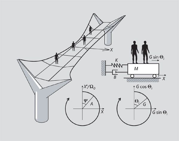
Figure 1. Taken from [2].
The left side of Figure 1 depicts the Millennium bridge. We are particularly interested in the lateral motion (i.e. side-to-side motion or sway) of the bridge.
For the modelling of the bridge, we can think about the bridge as a wheeled cart with mass M, see the top-right of Figure 1. This wheeled cart can only move in one dimension along the X-axis and this motion is representative of the sway of the bridge. The sway of the bridge is restricted by both stiffness and damping. A material is stiff if a force can only extend the material a little. Engineers like to think about stiffness as a spring where a stiff spring is hard to extend. If we go back to the picture of the cart in Figure 1, the quantity K represents the stiffness of the bridge. A damper is used by engineers to resist or to slow down motion. A common example of a damper in day-to-day life is a door closer which slows down a door so it will not slam. In the picture of the cart in Figure 1, the quantity B denotes damping where a larger B means more resistance.
With correctly chosen stiffness and damping, the sway of a bridge will eventually die down. If we simulate the lateral motion of bridge without pedestrians (which can be done with the simulation program which you will develop), we obtain the lateral displacement and lateral velocity in Figure 2 and you can see that their magnitudes become smaller over time.
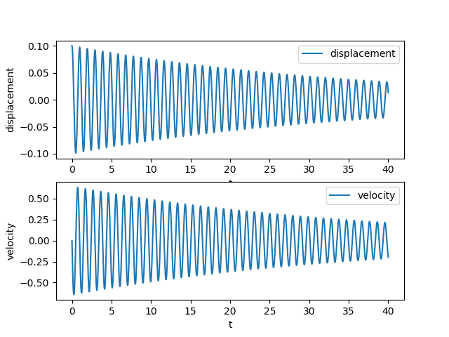
Figure 2. Displacement and velocity of the bridge without pedestrians
Since we will only consider lateral motion in this assignment, we will drop the word lateral for brevity from now on.
You can see from Figure 2 that the motion of the bridge is oscillatory. Engineers and scientists like to think about an oscillatory motion as a point going round in a circle. You can see how the motion of a circle maps to a sine curve here. We know that we can specify the position of a point on a circle by using an angle, so we can use an angle to describe the oscillatory motion of the bridge. This angle is commonly referred to as the phase angle or simply phase (in the same sense of the word "phase" in the expression "moon phase"). The bottom-centre picture in Figure 1 depicts an angle using the Greek alphabet Ψ (Psi). This angle is used to describe the phase of the oscillatory motion of the bridge.
The walking of a pedestrian can also described as a cycle since walking
is a repetition of: lifting of the left foot, landing of the left foot,
lifting of the right foot, landing of the right foot, and so on. For each
pedestrian, we can use a phase to describe their motion, see the angle Θ
i (Theta) in the bottom-right picture in Figure 1. Note that each
pedestrian on the bridge has his/her own phase, the subscript i in Θ
i is used to indicate the pedestrian whose index is i.
The theory in [2] is that the pedestrians synchronised their motion with that of the bridge. If we simulate the motion of the bridge with the pedestrians (which can be done with the simulation program which you will develop), we obtain the displacement and velocity in Figure 3 and you can see that their magnitudes grow over time. If you simulate for longer, the magnitude of oscillation will grow larger until it reaches a steady value.
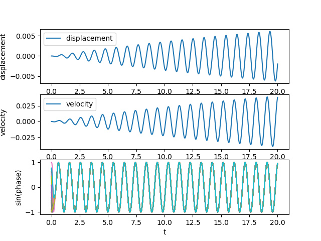
Figure 3. Displacement and velocity of the bridge with pedestrians
The bottom plot in Figure 3 shows the sine of the pedestrians' phase. There are 20 pedestrians and there are in fact 20 lines in different coloured lines in the plot. You can see the different coloured lines near time 0, but afterwards, these lines overlap and you can only see one coloured line. This means the pedestrians synchronised their walking.
Having seen that the displacement and velocity of the bridge will become large, a part of this assignment for you to see what modifications are needed to stabilise the bridge.
The above mental picture should give you the intuition you need for this assignment. In order to do simulation, we need a mathematical model which we will discuss next.A mathematical model for the bridge and pedestrians
From the bridge and pedestrian motion that we have discussed above, you know that we are interested in a few quantities:
- The displacement of the bridge at time t, which is denoted by x(t)
- The velocity of the bridge at time t, which is denoted by v(t)
- The phase of the bridge Ψ(t) at time t, which can be calculated from x(t), v(t), M and K. (Reminder: M is mass and K is stiffness)
- Each pedestrian's phase. We index the pedestrians by an index i where i takes on values from 0, ..., N-1 where N is the number of pedestrian on the bridge. At time t, the phase of the pedestrian i is denoted by Θi(t).
The mathematical model tells us how x(t), v(t), Ψ(t) and Θi(t) evolve over time.
The model has six model parameters. You have seen M, B, K and N before. There are two more: G and C. The table below summarises all the model parameters and their meaning. The Python programs will use the same notation for these model parameters.
| Constants | Meaning and their unit |
| M | Mass [kg] |
| B | Damping [kg/s] |
| K | Stiffness [kg/s/s] |
| N | Number of pedestrians |
| G | The maximum force that a pedestrian exerts on the bridge [N] |
| C | Larger C value means the pedestrians take shorter time to synchronise with the bridge [/m/s] |
We have placed the mathematical model for the bridge and pedestrians on a separate page. We believe it is best for you to get to know the different parts of the assignment before dwelling into the mathematical model. You should be able to get a big-picture understanding on what you need to do for this assignment without going into the mathematical model at this stage. (The model is here and you can read it later.) The mathematical model is modified from [2]. If you would like to read [2], click on this which will take you to the reference and there are links to download the paper.
Overview of tasks
We have divided the assignment into four tasks where each task corresponds to the writing of a Python function.
- Task 1 is to write the function sim_bridge() which simulates the bridge's displacement and velocity, as well as the pedestrians' phase
- The aim of Task 2 is to use the displacement and velocity of the bridge to compute a design objective. This design objective is such that, if the bridge oscillates more, then the design objective is bigger. In this task, you will write the function comp_obj().
- Assuming that it is possible to change the stiffness and damping of the bridge, you will use different values of stiffness and damping to see whether you can reduce the oscillation. You can do this because you have developed a simulation program. The aim of Task 3 is to develop the function run_different_designs().
- Now that you have got the different designs, the aim of Task 4 is to choose the best design. For this task, your aim is to write the function find_best_design().
Task 1: Simulation
The aim of this task is to write a Python function sim_bridge() to simulate the bridge and pedestrian motion. In the yellow box below, you can see some code for sim_bridge() which you can use to start your work.
| import
numpy as np def sim_bridge(t_array,M,B,K,G,N,C,Omega_array,dis0,vel0,ped0): # BEGIN: Supplied code ************************************ # Time increment dt = t_array[1] - t_array[0] # Initialise dis_array, vel_array, ped_array dis_array = np.zeros_like(t_array) vel_array = np.zeros_like(t_array) ped_array = np.zeros((N,len(t_array))) # Initialise for index 0 dis_array[0] = dis0 vel_array[0] = vel0 ped_array[:,0] = ped0 # Compute Y_0 [from eq 4] Y_0 = np.sqrt(K/M) # END: Supplied code ************************************ # Your code to compute the entries in dis_array, vel_array, ped_array # # Hint: Should use arctan2() from the numpy library to calculate Psi(t) # BEGIN: Supplied code ************************************ # Return the array return dis_array, vel_array, ped_array # END: Supplied code ************************************ |
The function sim_bridge() takes on a number of inputs. We will provide you with the parameter values to use so the important thing for you is to understand what they are referring to. The meaning of M, B, K, N, G and C have already been explained earlier at here. The meaning of the other inputs are explained in the table below.
| Python variable name | Meaning |
| t_array | A numpy array of regularly spaced points. They are the time instances in simulation. |
| Omega_array | This is a numpy array with N entries. The entry Omega_array[i]
is the value of Ωi in the mathematical model. The quantity Ωi is related to the walking speed of the the pedestrian with index i. We will explain how you can use Omega_array on the page where we describe the mathematical model. It is here and it is best that you read that later. |
| dis0 | Initial displacement of the bridge. This is a scalar. |
| vel0 | Initial velocity of the bridge. This is a scalar. |
| ped0 | This is a numpy array with N entries. The entry ped0[i] is the initial phase of the pedestrian with index i. |
The function sim_bridge() returns three outputs, see the second last line of the code above. All the three outputs are numpy arrays and their meanings are explained in the table below.
| Python variable name | Shape | Purpose |
| dis_array |
The same as t_array | To store the displacement of the bridge dis_array[j] is the displacement at the time given by t_array[j] |
| vel_array | The same as t_array | To store the velocity of the bridge vel_array[j] is the displacement at the time given by t_array[j] |
| ped_array | A two-dimensional numpy array The shape is N by the number of entries in t_array |
To store the phase of the pedestrians ped_array[i,j] is the phase of pedestrian i at the time given by t_array[j] |
Note that the template file has included code to create these three arrays with the specific shape mentioned above. Please do not change these lines of code. In addition, the template also includes lines of code which initialise these arrays for time 0. Again, please do not change these lines.
In order for you to complete sim_bridge(),
what you need to do is to add the for-loop for simulation.
(Testing and incremental development) You
can test this function by using the test file test_sim_bridge.py.
There are four test cases in this test file. We have developed these
test cases so that you can develop your sim_bridge()
incrementally. We will be explaining these test cases on a separate page
because it requires some understanding of the mathematical model. Our
suggestion is that you keep going with this document first to get an
understanding of the whole assignment. After that, you can read the
mathematical model and when you are ready to think about how to
implement sim_bridge(),
you can read how you can incrementally develop it on this
page, which is also where the mathematical model is.
Task 2: A function to calculate the design objective
The function sim_bridge() allows you to compute the displacement and velocity from the bridge parameters. In the next task (Task 3), you will explore different designs by varying the values of stiffness and damping. In order for us to choose a design later on, we need a way to measure how good a design is. This measure is known as the design objective. The aim of this task (Task 2) is to develop the function comp_obj() whose aim is to compute the design objective.
The def line of comp_obj() is:def comp_obj(dis_array,vel_array,M,K):
The names of the inputs have been chosen to reflect their roles. The function is expected to return one number as the design objective. We will use an example to explain how you compute the design objective.
(Example) Note that both dis_array and vel_array are expected to be 1-dimensional numpy arrays of the same shape. For this example, we assume:
- The entries of dis_array are [d0, d1, d2]
- The entries of vel_array are [v0, v1, v2]
We compute the following three numbers
square root of ( (d02 + (M / K) v02 ), square root of ( d12 + (M / K) v12 ), square root of ( d22 + (M / K) v22 )
where d02 denotes the square of d0 etc. The design objective is the maximum of these three numbers. In general, if there are H entries in each of dis_array and vel_array, you will be computing H numbers and finding the maximum of them.
As a numerical example, if
- dis_array is np.array([-1.1, 2.1, 3.1])
- vel_array is np.array([-4.1, -2.1, 1.3])
- K = 1.1
- M = 4.2
then you first compute
square root of ( (-1.1)2 + (M / K) (-4.1)2 ), square root of ( (2.1)2 + (M / K) (-2.1)2 ) , square root of ( (3.1)2 + (M / K) (1.3)2 )
Their numerical values are approximately 8.09, 4.61 and 4.01. The maximum is 8.09 which is the design objective. Your comp_obj() will need to return this number.
You can test this function by using test_comp_obj.py.
Note that it is possible to do all of the computation of this function
with merely one line of code in numpy. The lectures in Week 8 will give
you some inspiration.
Task 3: Calculating the design objective for many pairs of B
and K
Assuming that you are able to modify both the damping B and stiffness K of the bridge, you want to compute the design objective for many pairs of B and K values. The aim of this task is to develop the function run_different_designs() whose template is:
| def
run_different_designs( t_array, M,
G, N, C, Omega_array, dis0, vel0, ped0, B_min,
B_max, K_min, K_max, B_num, K_num): return B_array, K_array, sway_array |
There are many inputs to this function. The first group of inputs, which is typeset in blue, has been discussed before. The second group of inputs, which is typeset in maroon, is new.
This function returns three numpy arrays, see the return line in the
template code above.
In this task, you will use many different pairs of B and K values for simulation. For each pair of B and K, you will use sim_bridge() to obtain the displacement and velocity. (Note that you assume that the other parameters, M, G, N, ... remain the same.) Once the displacement and velocity have been obtained, you use them together with M and K to compute the design objective using comp_obj().
Note that the template file for run_different_designs() does not include default arguments. The last two parameters B_num and K_num can have default arguments. The default argument for B_num is 5, and that of K_num is 10. This is a piece of work that you need to complete for this task.
The steps inside the function run_different_designs() are:- Create a numpy array B_array of equally spaced values. The first and last values of this array are given, respectively, by B_min and B_max. The number of entries is determined by B_num. For example, if, at the time when the function is called, the specified values of B_min, B_max and B_num are, respectively, 11000.0, 27500.0 and 6, then B_array is expected to be array([11000., 14300., 17600., 20900., 24200., 27500.]). Note that the numbers in this array are equally spaced because the difference between any two consecutive entries is 3300. Note that if the value of B_num is not specified when the function is called, the default value of B_num, which is 5, should be used; in this case, we expect B_array to be array([11000., 15125., 19250., 23375., 27500.]).
- Create a numpy array K_array of equally spaced values. The first and last values of this array are given, respectively, by K_min and K_max. The number of entries is determined by K_num. Note that K_num has a default argument.
- Perform simulations for all possible pairs of B and K combinations that can be obtained from B_array and K_array. The number of possible B-K pairs is B_num times K_num. Let B_new and K_new be a particular pair of combination where B_new is an element in B_array and K_new is an element of K_array. For each pair of B_new and K_new, you need to do the following:
- Use B_new and K_new with the function sim_bridge() to compute the displacement dis_array and velocity vel_array when B_new is used as the damping and K_new is used as the stiffness. You can obtain the other inputs of sim_bridge() from the inputs to run_different_designs().
- Use the two arrays dis_array and vel_array computed in the last dot point, together with K_new and M to compute the design objective using comp_obj(). Note that M can be taken from the input.
- Let us assume B_new corresponds to the element with index i in B_array, i.e. the value of B_array[i] is B_new. Similarly, let us assume K_new corresponds to the element with index j in K_array. Store the design objective computed in the last dot point in the array element sway_array[i,j]. Note that the shape of sway_array is expected to be B_num by K_num .
You can use the file test_run_different_designs_0.py,
test_run_different_designs_1.py
and test_run_different_designs_2.py
to test
your function. Note that for both test_run_different_designs_0.py,
test_run_different_designs_1.py,
the
value of B_num
by K_num
are specified. For test_run_different_designs_2.py,
both B_num
by K_num
are not specified so the default arguments are expected to be used.
Note that for all these three test files, a number of simulations will be run so the computation may take a bit of time. The files test_run_different_designs_0, test_run_different_designs_1 and test_run_different_designs_2 run, respectively, 12, 24 and 50 different designs. If you need computing power, you can use a vlab computer.
Hint: You will need to use nested-for for this function. An example of using nested-for can be found in the file nested_for.py in Week 5B.
Remark: We
want to remark that the design problem that we have posed above is not
entirely realistic. It is hard to modify the stiffness of a bridge, see [1].
If stiffness and damping are modified, the other bridge parameters, such
as the mass M, may need to be adjusted at the same time. We have taken the
liberty to keep the problem simple.
Task 4: Choose the best design
The aim of this task is to choose the best design from all those designs that you have simulated in Task 3. In this assignment, we define the best design as the pair of B and K that minimises the design objective. In this task you will develop the function find_best_design() whose template is:
| def
find_best_design(sway_array,B_array,K_array): return B_chosen, K_chosen |
The inputs sway_array, B_array and K_array are the outputs of run_different_designs(). The function is expected to return two outputs which are the chosen pair of B and K.
Let us use an example to illustrate the expected behaviour of find_best_design(). For this example, we assume that sway_array, B_array and K_array are given by:
| sway_array
= np.array( [ [3.1, 2.1, 1.1], [4.1, 1.6, 2.4], [2.2, 3.2, 3.6], [1.5, 2.5, 3.5] ] ) B_array = np.array([3.7, 4.7, 5.7, 6.7]) K_array = np.array([1.5, 1.8, 2.1]) |
Note that B_array has 4 entries, K_array has 3 entries, and from run_different_designs() we expect that sway_array should have a shape of (4,3). Recall also that sway_array[i,j] is computed from B_array[i] and K_array[j], e.g. sway_array[2,1] , which has the value of 3.2 (highlighted in blue), is the design objective computed by using B_array[2] and K_array[1].
Since our goal is to find the design that minimises the design objective, we look for the smallest element in sway_array, which is sway_array[0,2] and has a value of 1.1 (highlighted in magenta). The best design therefore comes from a value of B equals to B_array[0] and a value of K equals to K_array[2]. You should assign B_array[0] to B_chosen and K_array[2] to K_chosen.
You can test find_best_design() by using the test file test_find_best_design().
Note that you can use numpy to write this function without using any loops.
Remark: We have used a rather brute force method to determine the design parameters. You will learn better optimization methods in later years.
Putting all functions into action
We have provided you with a Python program called run_all.py. In this file, you will use run_different_designs() to simulate a number of different designs and use find_best_design() to choose the best design. After that, the file will use sim_bridge() to simulate the bridge, first with the original parameters and then with new parameters obtained from the design. If your programs work correctly, you should be able to see that the new design has stabilised the bridge.
This is not part of the assessment but we think it is good for you to see how you can put everything together.
Getting Started
- Download the zip file assign2_prelim.zip, and unzip it. This will create the directory (folder) named 'assign2_prelim'.
- Rename/move the directory (folder) you just created named 'assign2_prelim' to 'assign2'. The name is different to avoid possibly overwriting your work if you were to download the 'assign2_prelim.zip' file again later.
- First browse through all the files provided including the test files.
- (Incremental development) Do not try to implement too much at once, just one function at a time and test that it is working before moving on.
- Start implementing the first function, properly test it using the given testing file, and once you are happy, move on to the the second function, and so on.
- Please do not use 'print' or 'input' statements. We won't be able to assess your program properly if you do. Remember, all the required values are part of the parameters, and your function needs to return the required answer. Do not 'print' your answers.
The zip file assign2_prelim.zip contains altogether 23 files. The assumption is that all these 23 files must be in same directory. Here is an overview of what the files are:
- 4 template files for the 4 functions to be written
- <6 test files for the four functions to be written.
- 2 files with the extension txt which are needed to run the
simulation. The test files have code to handle these two files so
you do not have to worry about them.
- 10 files with the extension npz. We have pre-computed the expected
results and store them in these files. The test files will load
these files and compare the expected results against your results.
- run_all.py as an example on how to put all the files together.
Testing
Test your functions thoroughly before submission.
You can use the provided Python programs (files like test_sim_bridge.py
etc.) to test your functions. Please note that each file covers a limited
number of test cases. We have purposely not included all the cases
because we want you to think about how you should be testing your code. You
are welcome to use the forum to discuss additional tests that you should
use to test your code.
The test files will calculate the
difference between the expected results and your results. The test
file will inform you the maximum absolute difference. The difference
should be less than 1e-6.
We will test each of your files independently. Let us give you an example. Let us assume we are testing three files: prog_a.py, prog_b.py and prog_c.py. These files contain one function each and they are: prog_a(), prog_b() and prog_c(). Let us say prog_b() calls prog_a(); and prog_c() calls both prog_b() and prog_a(). We will test your files as follows:
- We will first test your prog_a().
- When we test your prog_b(), we will test your prog_b() together with our working version of prog_a(). In this way, if your prog_a() does not work for some reason, there is a chance that your prog_b() may work and you may still receive marks for prog_b().
- When we test your prog_c(), we will test your prog_c() together with our working version of prog_a() and prog_b().
Submission
You need to submit the following four files. Do not submit any other files. For example, you do not need to submit your modified test files.
- sim_bridge.py
- comp_obj.py
- run_different_designs.py
- find_best_design.py
To submit this assignment, go to the Assignment 2 page and click the tab named "Make Submission".
Assessment Criteria
We will test your program thoroughly
and objectively. This assignment will be marked out of 24 where 20 marks
are for correctness and 4 marks are for style.
Correctness
The 20 marks for correctness are awarded according to these criteria.
| Criteria | Nominal marks |
| Function sim_bridge() (Case 0: G = 0, C = 0, non-zero initial conditions. Need to get dis_array and vel_array correct) | 2 |
| Function sim_bridge() (Case 1: nonzero G. C = 0. Need to get dis_array, vel_array and ped_array correct) | 3 |
| Function sim_bridge() (Case 2: nonzero G and C. Need to get dis_array, vel_array and ped_array correct) | 4 |
| Function comp_obj() | 2 |
| Function
run_different_designs() (Case 0: All arguments are specified. No
default arguments will be used.) |
4 |
| Function run_different_designs() (Case 1: Testing default arguments.) | 1 |
| Function find_best_design() | 3 |
(Assessment and incremental development) We told you earlier that the function sim_bridge() can be developed incrementally, which are Step 0, Step 1 and Step 2 mentioned here. Each step corresponds to a more complicated simulation model with Step 0 being the simplest and Step 2 being the complete model. We want to let you know that there is a one-to-one correspondence between the incremental development of sim_bridge() and the assessment of sim_bridge(). The assessment of sim_bridge() is divided into 3 cases, see the table above. Case 0 in the assessment corresponds to Step 0 of the incremental development, and so on. You need to know.
- You can still get marks for partially completed simulation models, i.e. completing Step 0 or Step 1.
- You do not have to get all three Steps going before working on the other functions. Note that:
- The test file test_run_different_designs_0.py assumes that you have got Step 0 of the simulation model working
- The test file test_run_different_designs_1.py assumes that you have got Step 1 of the simulation model working
- The test file test_run_different_designs_2.py assumes that you have got Step 2 of the simulation model working
The important message is this: Just in case you find doing the simulation model difficult, you can get a partially completed simulation model going first and then move on to work on the other functions first. Do not think that you need to complete the entire simulation model before working on the other functions.
Style
Four (4) marks are awarded by your tutor for style and complexity of your solution. The style assessment includes the following, in no particular order:- Use of meaningful variable names where applicable
- Use of sensible comments to explain what you're doing
- Use of docstring for documentation to identify purpose, author, date ,
data dictionary, parameters, return value(s) and program description at
the top of the file
Assignment Originality
You are reminded that work submitted for assessment must be your own. It's OK to discuss approaches to solutions with other students, and to get help from tutors, but you must write the Python code yourself. Sophisticated software is used to identify submissions that are unreasonably similar, and marks will be reduced or removed in such cases.
Assignment Conditions
- Joint work is not permitted on this assignment.
This is an individual assignment. The work you submit must be entirely your own work: submission of work even partly written by any other person is not permitted.
Do not request help from anyone other than the teaching staff of ENGG1811 - for example, in the course forum, or in help sessions.
Do not post your assignment code to the course forum. The teaching staff can view code you have recently submitted.
Assignment submissions are routinely examined both automatically and manually for work written by others.
Rationale: this assignment is designed to develop the individual skills needed to produce an entire working program. Using code written by, or taken from, other people will stop you learning these skills. Other CSE courses focus on skills needed for working in a team.
- The use of code-synthesis tools, such as GitHub Copilot, is not permitted on this assignment.
Rationale: this assignment is designed to develop your understanding of basic concepts. Using synthesis tools will stop you learning these fundamental concepts, which will significantly impact your ability to complete future courses.
-
Sharing, publishing, or distributing your assignment work is not permitted.
Do not provide or show your assignment work to any other person, other than the teaching staff of ENGG1811. For example, do not message your work to friends.
Do not publish your assignment code via the Internet. For example, do not place your assignment in a public GitHub repository.
Rationale: by publishing or sharing your work, you are facilitating other students using your work. If other students find your assignment work and submit part or all of it as their own work, you may become involved in an academic integrity investigation.
- Sharing, publishing, or distributing your assignment work after the completion of ENGG1811 is not permitted.
For example, do not place your assignment in a public GitHub repository after this offering of ENGG1811 is over.
Rationale: ENGG1811 may reuse assignment themes covering similar concepts and content. If students in future terms find your assignment work and submit part or all of it as their own work, you may become involved in an academic integrity investigation.
Violation of any of the above conditions may result in an academic integrity investigation, with possible penalties up to and including a mark of 0 in ENGG1811, and exclusion from future studies at UNSW. For more information, read the UNSW Student Code, or contact the course account.
Further Information
- We will run Help Sessions for this assignment during Weeks 8-10.
- Use the forum to ask general questions about the assignment, but take specific ones to Help Sessions or post as Private.
- Keep an eye on the course webpage notice board for updates and responses.
Reference
[1] T. Fitzpatrick and R. R. Smith. Stabilising the London Millennium Bridge. Ingenia online pdf at (https://www.ingenia.org.uk/getattachment/Ingenia/Issue-9/Stabilising-the-London-Millennium-Bridge/Fitzpatrick.pdf)
[2] Strogatz, S. H., Abrams, D. M., McRobie, A., Eckhardt, B. & Ott, E. 2005 Crowd synchrony on the Millennium Bridge. Nature 438. (doi:10.1038/43843a). Links to the paper and its supplementary information.
[3] J. H. G. MacDonald. Lateral excitation of bridges by balancing pedestrians. Proc. of Royal Society A. (2009)